k-Nearest Neighbour Astro example: 2D Photometric Completeness Map

Astronomical research which uses CCD photometry typically requires that the photometric depth of the field be accurately determined. One common statistic to describe a field is the magnitude at which 50% of the objects are recovered. So if you had 100 objects at this brightness (magnitude) you'd statistically expect that about 50% of them would be recovered by your detection algorithm. Fainter than this point the detection algorithm typically rapidly decays until you reach a magnitude where almost no stars are recovered.

The most common way to describe this decay in the amount of stars recovered is to use a Logisitic function. While typical usage of the logistic function has it going from 0 to 1, in astronomy, we normally use the inverse logistic function such that it goes from 1 to 0.

To test the depth of the data we have injected artificial stars across the field and then using the same detection algorithm that was used on the real stars, we determine how well we can recover these fake stars. For this example, we have employed 500,000 artificial stars spread randomly across the field and distributed in colour and magnitude space to reflect the nature of the original dataset.

In this figure, I show how the photometric completeness for the entire field can be fit with a logistic function.

Making the Map

Because we so many artificial stars and because they are spread randomly across the field and randomly in colour-magnitude space, each artificial star will have, in its vicinity, enough local stars to construct simple version of the photometric completeness profile as see in the figure above.

This means we can make an estimate of the local completeness by sampling those "local" artificial stars in our region of interest.

To do this, we're going to use the k-Nearest Neighbours package from sklearn in Python.

k-Nearest Neighbours

In this example, I'm taking advantage of the "Nearest Neighbours" routine from sklearn to streamline my code in what otherwise could be done using the Euclidean distance between the points. We could set a radial distance for example and select object inside that but when determining a decent completeness profile, it's important to have well populated bins. The risk with a simple radial search is that in the corners or near the edges signficant numbers of objects will be lost due to the geometry. By using the kNN search we can easily overcome this problem, although it does mean those locations will be more heavily smoothed by this approach than the interior of the field.

In the code, we have two subroutines:

• completeness: which builds the completeness histogram which we would normally fit with a logistic function The version we use here is the ratio (per input bin) of stars recovered/input.
• findmidpoint: which takes the output of "completeness" and interpolates the precise point of the 50% level.

Note: For the purpose of the example below, I assume that that around the 50% point, the logistic function is essentially linear and I fit a line across the midpoint and interpolate the "true" 50% level.

The data consists of photometry in the g-band ("blue" filter) and the r-band ("red" filter) and we'll determine how the 50% level looks in both cases.

The Code

Coding Efficiency Issues**

So it's fairly clear upon close inspection of the code that running a do loop on 500,000 objects is going to be slow and undesirable (which it is). At this stage, I'm not sure what the work around for that is, especially since, I need to find the k-Nearest Neighbours around each point and this hard to do with a single big matrix operation. So for the time being, just sleep on it while it crunches its way through the file. Comments welcome.

Reading in the data

Often examples for how to use a routine are built upon artificially generated data, in this case you can see that we're reading in a text file, with columns and moving forward from there.

import numpy as np
from sklearn.neighbors import NearestNeighbors
import matplotlib.pyplot as plt

#+++ read in the data file +++++++++++++++++++++++++++++++++++++++++++++++++++++#

## read in the data here, in my example it is a table of 500,000 objects with a column for each variable ##
names='fake_ext fake_chip fake_xpix fake_ypix fake_counts_g fake_g fake_counts_r fake_r ext chip xpix ypix chi snr sharp roundness majaxis crowding objtype \
counts_g sky_g norm_counts_g norm_counts_g_err mag_inst_g mag_inst_g_err \
chi_g snr_g sharp_g round_g crowd_g fwhm_g ecc_g psfa_g psfb_g \
psfc_g flag_g counts_r sky_r norm_counts_r norm_counts_r_err mag_inst_r mag_inst_r_err chi_r \
snr_r sharp_r round_r crowd_r fwhm_r ecc_r psfa_r psfb_r psfc_r flag_r newgmag newrmag'.split()

data=np.genfromtxt(filename,names=names,dtype=None).view(np.recarray)

Subroutines to help us build the maps

As discussed above, these are the two subroutines, one which bins the data to form the completeness profile and the other to find the midpoint which we'll store and plot later. Note also that I'm doing both filters together, this could also be made more general with two calls to completeness instead of one.

Note that the midpoint routine has a little if statement to check which side of the true midpoint we actually are before proceeding.

def completeness(gmag, rmag, snr_g, snr_r, sharp_g, sharp_r, g_err, r_err, objtype):
    step = 0.1
    mag_bins_g = np.array(np.arange(gmag.min(), gmag.max(), step))
    ref_hist_g = np.zeros(np.size(mag_bins_g))
    hist_g = np.zeros(np.size(mag_bins_g))

    mag_bins_r = np.array(np.arange(gmag.min(), gmag.max(), step))
    ref_hist_r = np.zeros(np.size(mag_bins_r))
    hist_r = np.zeros(np.size(mag_bins_r))
    ## fill the bins

    #quality cuts, to select good stars

    qcuts= ( (snr_g >= 3.5) & ((sharp_g*sharp_g <= 0.1) | (sharp_r*sharp_r <= 0.1)) & (snr_r >= 3.5)  & (g_err<9.) &\
    (r_err<9.) & (objtype == 1) )#& (data.flag_g == 0) & (data.flag_r == 0)) #


    ref_g, binsg = np.histogram(gmag,mag_bins_g)
    ref_r, binsr = np.histogram(rmag,mag_bins_r)

    hist_g, binsg = np.histogram(gmag[qcuts],mag_bins_g)
    hist_r, binsr = np.histogram(rmag[qcuts],mag_bins_r)

    complete_g = hist_g.astype(float)/ref_g.astype(float)
    complete_r = hist_r.astype(float)/ref_r.astype(float)

    x0 = binsg[:-1]+step/2.0
    data0 = complete_g

    x1 = binsr[:-1]+step/2.0
    data1 = complete_r

    return x0, x1, data0, data1

def findmidpoint(x0, x1, data0, data1):

    #g_n is the mag closest to the 50% level
    #comp_n is that value
    gm50 = np.argmin(abs(data0-0.5))
    g_n = x0 #x
    comp_n = data0 #y

    rm50 = np.argmin(abs(data1-0.5))
    r_n = x1 #x
    comp_n = data1 #y


    if (data0[gm50]< 0.5):

        m = ( comp_n[gm50+1] - comp_n[gm50] )/ (g_n[gm50+1] - g_n[gm50])
        b = comp_n[gm50] - m*g_n[gm50]

        g_50 = (0.5 - b)/m

    else:

        m = ( comp_n[gm50] - comp_n[gm50-1] )/ (g_n[gm50] - g_n[gm50-1])
        b = comp_n[gm50] - m*g_n[gm50]

        g_50 = (0.5 - b)/m

    if (data1[rm50] < 0.5):

        m = ( comp_n[rm50+1] - comp_n[rm50] )/ (r_n[rm50+1] - r_n[rm50])
        b = comp_n[rm50] - m*r_n[rm50]

        r_50 = (0.5 - b)/m

    else:

        m = ( comp_n[rm50] - comp_n[rm50-1] )/ (r_n[rm50] - r_n[rm50-1])
        b = comp_n[rm50] - m*r_n[rm50]

        r_50 = (0.5 - b)/m

    return g_50, r_50

Main Code

So here we need to do a little data manipulation by zipping the x and y pixel locations together. We also do a bit of admin code, by building the arrays to hold the solutions. You might also like to note the somewhat annoying reshaping of the array that has to occur to get the indices of the nearest neighbours.

For the time being, I'm plotting this up in TopCat, so I just dump the data to a text file.

XX = np.array(zip(data.fake_xpix,data.fake_ypix))

blocks = np.size(data.fake_xpix) #500,000

g50s = np.zeros(blocks)
r50s = np.zeros(blocks)
kNN = 20000

nbrs = NearestNeighbors(n_neighbors=kNN, metric='euclidean').fit(XX)

for i in range(blocks):

    distances, indices = nbrs.kneighbors(XX[i].reshape(1,-1))

    newbinsg, newbinsr, newcomp_g, newcomp_r = completeness(mag1[indices], mag2[indices], data.snr_g[indices], data.snr_r[indices], data.sharp_g[indices], data.sharp_r[indices], data.mag_inst_g_err[indices], data.mag_inst_r_err[indices], data.objtype[indices])

    g50, r50 = findmidpoint(newbinsg, newbinsr, newcomp_g, newcomp_r)

    g50s[i] = g50
    r50s[i] = r50


Resultsoutput = np.transpose((np.vstack((XX[:,0],XX[:,1], g50s, r50s))))

np.savetxt('test50s_v2.txt', Resultsoutput,fmt='%.3f')

Plotting with TopCat

Sometimes doing something quick does not mean it is necessarily dirty.

Instead of faffing with matplotlib and meshgridding half a million points, I'm going to jump to another tool. Here I've taken the output text file with the results and loaded them into the Java package TopCat for plotting. TopCat is a very handy tool for quickly appraising astronomical data and doing preliminary data analysis, cross-matching, conversions and much more.

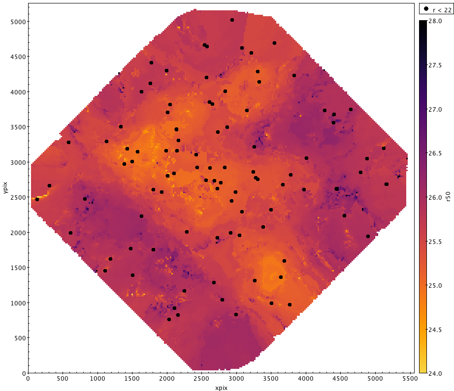
In our case, we want it to make a nice plot where we use the 50% level (g50 or r50) as an auxilliary axis to colour code the data. While we could just plot it as points, it will look much nicer if we use the "density form" and bin the data a little to ensure there are no gaps in the plotting. Each of these new pixels is the median of the points that fall in that bin. To avoid outliers from washing out any substructure, we limit the range to $\pm$ 1.5 mags of the expected value.

What is then revealed is a map of how the photometric completeness varies across the field. I've also overplotted the location of the brightest stars in the field as black dots for reference.